A Beginner's Perspective on Dynamical Systems
Introduction to Dynamical Systems
Dynamical systems provide a mathematical framework to study how things change over time(dynamical). This blog aims to introduce the basic concepts and tools used to analyze 1-dimensional and 2-dimensional systems.
When I first encountered dynamical systems, I was incredibly confused. We already have Cartesian space, partial differential equations (PDEs), and ordinary differential equations (ODEs) to describe trajectories in Cartesian space—so why do we need phase space? Isn’t Cartesian space enough?
As I delved deeper into the subject, I realized the limitation of describing dynamics solely in Cartesian space: it lacks temporal information, and maybe this is where the word dynamical stands for.
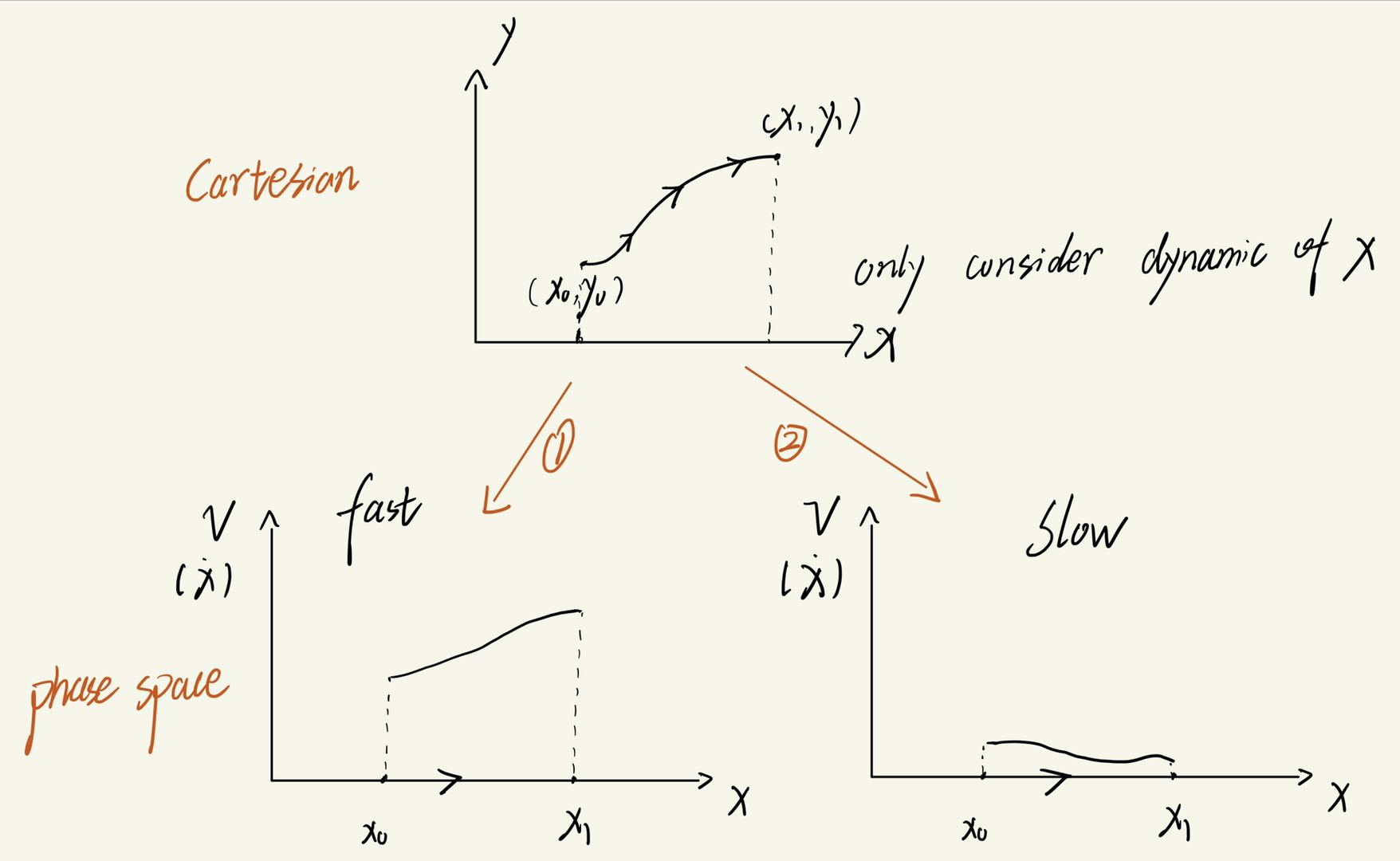
Consider the figure above, which shows a trajectory in 2D Cartesian space. A point moves from $(x_0,y_0)$ to $(x_1,y_1)$. While we can see the path the point takes, we have no way to tell how fast it moves along that path. The trajectory alone doesn’t reveal the system’s velocity or how it evolves over time.
This is where phase space becomes essential. By transitioning to phase space, we can visualize not only the position of the system but also its velocity (or momentum, depending on the context) at every point. For instance, in phase space, we can represent a system’s state using both $x$ and its velocity $ v=\dot{x} $ .This allows us to observe how the dynamics evolve over time with greater clarity.
Figures $ 1 $ and $2$ in phase space illustrate that two different dynamics can share the same trajectory in Cartesian space.
By visualizing the velocity at each position, phase space provides a richer, more complete picture of the system’s behavior. It becomes a powerful tool for studying how trajectories change, identifying patterns like fixed points, limit cycles, or chaotic behavior, and understanding the system’s overall dynamics.
1. One-Dimensional Flow
Let’s begin with a one-dimensional system. The first unfamiliar notation you’ll likely encounter in dynamical systems is $ \dot{x} $. But don’t worry—it’s simply another way of writing $\frac{dx}{dt}$. Typically, we express this as $ \dot{x}= f(x) $, which means that for every value of $x$, the system has a corresponding rate of change $\frac{dx}{dt}= f(x)$. For example, if $x$ represents position, then $ \dot{x}= f(x) $ describes the velocity at that specific position.
1.1 Fixed Points
- Definition: Points where the system does not change over time $ \dot{x} = 0 $.
- Examples of fixed points in simple systems.
1.2 Linear stability analysis
This is a very useful technique to expand the flow around fixed point, so that we can observe how higher order term dictates the dynamic around the fixed point.
A general flow $ \dot{x} = f(x) $ can be solved close to any fixed point $ x = x^* $. A small deviation $ \eta(t) = x(t) - x^* $ from $ x^* $ evolves according to
\(\dot{\eta} = \dot{x} - \frac{d}{dt} x^* = \dot{x} = f(x)\)
Series expand the flow around the fixed point to linear order:
\(\dot{\eta} = f(x) = \underbrace{f(x^*)}_{=0} + f'(x^*) \underbrace{(x - x^*)}_{=\eta} + \frac{1}{2} f''(x^*) \underbrace{(x - x^*)^2}_{=\eta^2} + \cdots\)
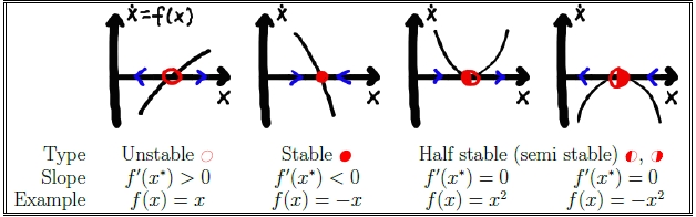
where $f(x^*) = 0 $ ($ \frac{d}{dt}x^*=0 $) accordingto the definition of a fixed point. Solution: \(\eta = \eta_0 e^{f'(x^*)t}\)
stability exponent: $\lambda = f’(x^*)$ is the stability exponent,It determines whether the fixed point is stable (λ < 0) or unstable (λ > 0).
be careful! the stability exponent is not $\lambda = \ddot{x}$ . This is incorrect because it means$ \ddot{x} = \frac{d^2 x}{dt^2} $, while the stability exponent is the derivative of $ \dot{x} $ with respect to the coordinate $ x $, $ \lambda \equiv \frac{\partial \dot{x}}{\partial x} $.
1.3 Bifurcations in 1D
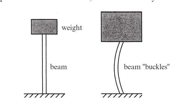
What is bifurcation? A bifurcation is a qualitative change in the dynamics of a system as a parameter is varied. Imagine a box resting on a pole. As the weight of the box changes, the curvature of the pole also changes to balance the system. However, if we keep increasing the weight of the box, there may come a point where the pole breaks. This breaking point represents a bifurcation in the box-pole system: beyond this point, the pole can no longer return to any stable curvature, regardless of the weight of the box.
- One-Parameter Bifurcations:
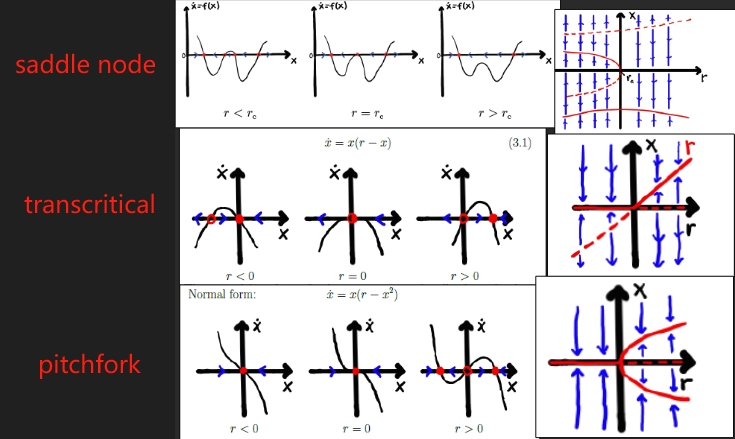
- Saddle-node bifurcation.
- Transcritical bifurcation.
- Pitchfork bifurcation (supercritical and subcritical).
- Two-Parameter Bifurcations:
- In systems with two parameters $r$ and $s$,$ \dot{x} = f(x, r, h)$ , fixed points form surfaces
$x^*(r, h)$all the points on the surface are where $\dot{x}=0$ so the surface also called equilibrium manifold , and bifurcations occur at curves $h_c (r)$. when $h=0$ we can imagine on $xor$ (in the plot the $u$ should be $x$ here, never mind≧▽≦) plane will form a supercritical pitchfork, and when $r>0$ there will be 3 fixed points.
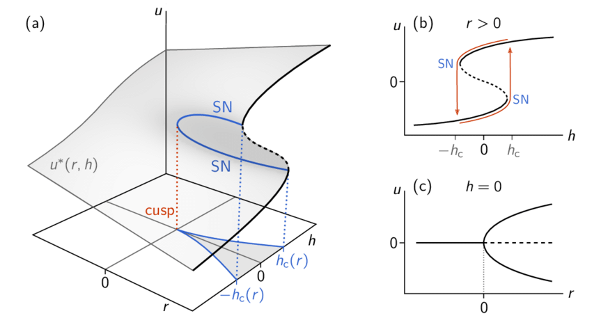
- catastrophe:A small change in a parameter that causes a significant change in the equilibrium state of a system.
- hysteresis: The loop in the $xoh$ plane is called hysteresis loop, a small change of $h$ near $h_c$ will lead to a drastic change of equilibrium state, and if the system want to return to the equilibrium state before, $h$ should be adjust to $-h_c$ and then slowly adjust back to $h_c$.
- In systems with two parameters $r$ and $s$,$ \dot{x} = f(x, r, h)$ , fixed points form surfaces
$x^*(r, h)$all the points on the surface are where $\dot{x}=0$ so the surface also called equilibrium manifold , and bifurcations occur at curves $h_c (r)$. when $h=0$ we can imagine on $xor$ (in the plot the $u$ should be $x$ here, never mind≧▽≦) plane will form a supercritical pitchfork, and when $r>0$ there will be 3 fixed points.
2. Flow on the Plane
Flow in the plane is far more intriguing than in 1D, as it exhibits a richer global structure. Instead of a single fixed point, you can encounter phenomena such as closed orbits, limit cycles (isolated closed orbits), and homoclinic or heteroclinic orbits, among others.
2.1 Fixed Points in 2D
- Classification using Linear Stability Analysis: For a 2D system, we begin by determining its Jacobian matrix. Specifically, near the fixed point we wish to analyze, we use a linear approximation to study the dynamics in its vicinity.
and the fixed points type can be classfied as below:
- Stable/unstable spiral.
- Stable/unstable node.
- Center.
- Degenerate.
By referencing the ‘Zoo’ of fixed points, one can quickly determine the type of a fixed point using the trace and determinant of the Jacobian matrix.
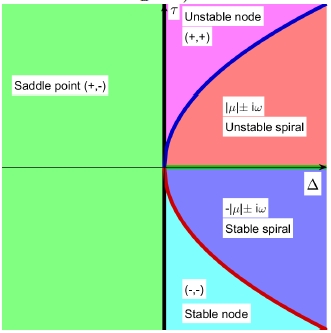
For a 2D system \(\dot{x} = Ax \, , \, A = \begin{bmatrix} a & b \\ c & d \end{bmatrix} \, .\) according to the characteristic equation $0 = \det(A - \lambda I) = \lambda^2 - \tau\lambda + \Delta$( where $\tau = a + d$, namely the Trace of the matrix, and $\Delta = ad - bc$ which is the determinant of the matrix), we can get the eigenvalues of the system.
Why are we interested in the eigenvalues of the system? Because they allow us to transform the system so that its eigenvectors are aligned with the coordinate axes. This simplifies the analysis, as we can focus on how the eigenvalues dictate the system’s behavior near the fixed point. If the real part of an eigenvalue is greater than 0, the system expands exponentially along the corresponding eigenvector direction. Conversely, if the real part of an eigenvalue is less than 0, the system contracts exponentially along that direction.
The proof below demonstrates that eigenvalues act as the exponents in the solution trajectories, explaining the origins of exponential expansion and contraction.
$$ \dot{x}=Ax = PDP^{-1}x \\ \Rightarrow \frac{d}{dt}[P^{-1}x] = D \underbrace{P^{-1}x}_{\xi} \\\Rightarrow \dot{\xi} = D\xi \\ \Rightarrow \xi(t) = \begin{pmatrix} e^{\lambda_1 t} \xi_1(0) \\ e^{\lambda_2 t} \xi_2(0) \end{pmatrix}$$
When I first learned this, I was confused about why zero is the threshold and not one. I initially thought that repeatedly applying a matrix to a given vector would cause the vector to grow in the direction where $|\lambda|>1$ and shrink in the direction where $|\lambda|<1$.
My misunderstanding arose because the matrix is not directly applied to a physical entity but rather operates in the phase space, specifically on the ODE system. When solving the ODE system to obtain the solution, $\lambda$ represents the exponent rather than a multiplier!
And this is where oscillations come into play!!when eigenvalues are complex, the solution looks like this \(\xi(t) = \xi_1(0) e^{\mu t} \begin{pmatrix} \cos(\omega t) \\ \sin(\omega t) \end{pmatrix}\), where $\mu$ is the real part and $\omega$ is the complex part of the eigenvalues.
2.2 Non-Local Structures
Thus far, we have only discussed the local behavior of a system around a specific point, namely a fixed point. However, in 2D systems, new structures such as closed orbits and limit cycles can also emerge.
- Closed Orbits in Hamiltonian Systems:
- Conservation laws leading to closed orbits.
- A simple Hamiltonian system like this can form closed orbits in the phase space plane. Imagine bands of closed orbits surrounding the center, representing trajectories corresponding to different initial speeds given to the box at the same starting position.
- The mathematic form of a Hamiltonian system would be like this:
$$ H \equiv \frac{p^2}{2m} + V(x) \\ \dot{x} = \frac{\partial H}{\partial p} = \frac{p}{m} \\ \dot{p} = -\frac{\partial H}{\partial x} = -\frac{\partial V}{\partial x} \\$$
Here, $x$ typically represents the position, while $p$ denotes the momentum, defined as $p=mv$. So the total energy $E=H(x,p)$ is conserved since $\dot{H}=0$, namely the total energy will not change over time.
$$\dot{H} = \frac{\partial H}{\partial x} \underbrace{\dot{x}}_{\frac{\partial H}{\partial p}} + \frac{\partial H}{\partial p} \underbrace{\dot{p}}_{-\frac{\partial H}{\partial x}} = 0.$$
-
Limit Cycles:
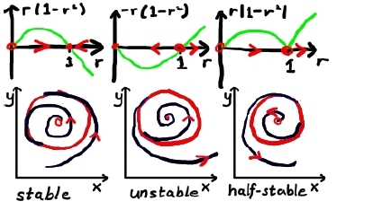
In systems without symmetry, bands of closed orbits are rare since non-linearity generally destroys centers. However, oscillations can still occur through formation of isolated closed orbits, known as limit cycles.
It is often easier to analyze circular structures using polar coordinates. A typical limit cycle can form in a system like this.
- How to find limit cycles:
- Poincaré-Bendixson Theorem:Assume a smooth flow in a bounded domain D of the plane. Assume further that D does not contain any fixed point and that there exists a trajectory that is confined in D for all times. Then at least one periodic orbit exists in D.
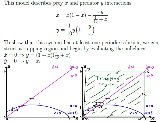
- Poincaré-Bendixson Theorem:Assume a smooth flow in a bounded domain D of the plane. Assume further that D does not contain any fixed point and that there exists a trajectory that is confined in D for all times. Then at least one periodic orbit exists in D.
- How to rule out closed orbits or limit cycles
- Gradient systems: $\dot{x} = - \nabla V(x)$ , in gradient systems $x$ always move toward the direction decrease total energy $V$ the most, so there would be no oscillations.
- Dulac’s criterion:consider a differentiable function $V (x)$ such that $\nabla · (V\dot{x})$ does not change sign in some domain. If such function exists, there are no closed orbits in the domain (Green’s theorem).
- Index theory : The index of a limit cycle is always +1. Therefore, if the index of a closed curve is −1 and we can confirm there is only one fixed point within the region, we can conclusively rule out the existence of a limit cycle inside.(and there more other rules like this. this just one of them.)
- How to find limit cycles:
2.3 Bifurcations of Limit Cycles
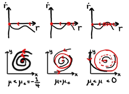
- Saddle-node bifurcation of limit cycles: just change r, and the limit cycle will come out from no where!
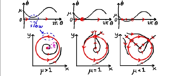
- SNIPER (Saddle-Node Infinite Period) bifurcation. Adjust the angular velocity $\omega$until, at a certain point, a fixed point emerges precisely on the limit cycle.
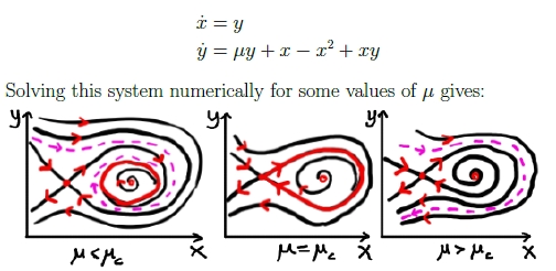
- Homoclinic bifurcation: Collision between a limit cycle and a saddle point!
2.4 Planar Bifurcations
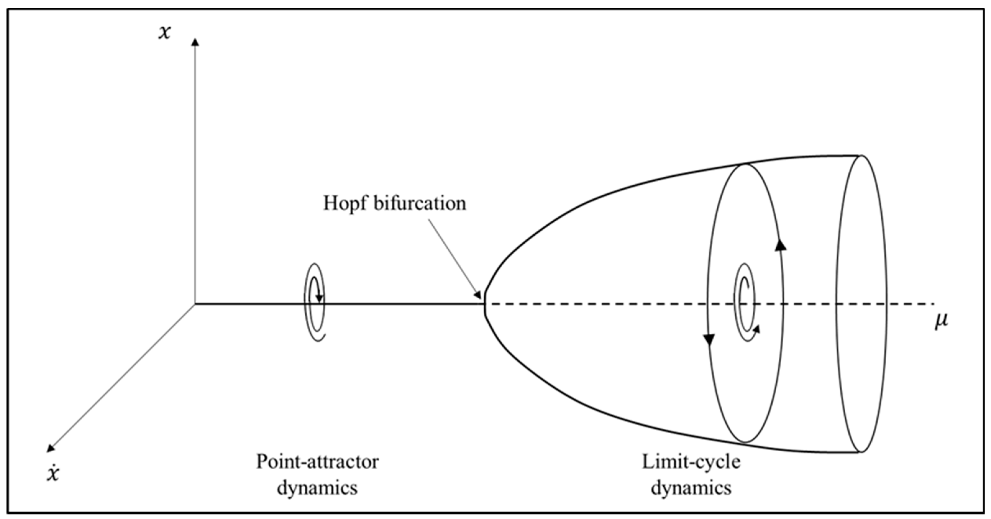
Aside from the bifurcation of limit cycles in the phase plane, another type of bifurcation that can occur in 2D systems is the Hopf bifurcation.
- Hopf Bifurcation:
- Supercritical Hopf bifurcations: can be visualized as a limit cycle ‘growing out’ from a fixed point. This type of bifurcation occurs when a change in parameters causes a transformation in the ‘Zoo’ of dynamical behaviors, as described in Section 2.1.
- Supercritical Hopf bifurcations: can be visualized as a limit cycle ‘growing out’ from a fixed point. This type of bifurcation occurs when a change in parameters causes a transformation in the ‘Zoo’ of dynamical behaviors, as described in Section 2.1.
2.5 Index Theory
Poincaré Index of a vector field in the plane is an integer that describes global information about the phase portrait around isolated singular points. The value of the index is determined by how the vector field orients around the singular points.
- Introduction to the Poincaré Index:
- The index of any closed, non-intersecting curve C not passing through any fixed point is defined as the winding of a vector field as we traverse one counter-clockwise lap on C:
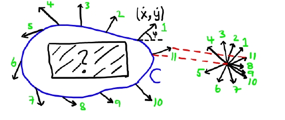
- We can also solve it analytically, but be cautious: $\varphi =\text{atan} \left( \frac{\dot{y}}{\dot{x}} \right)$ but not $\varphi =\text{atan} \left( \frac{y}{x} \right)$ . This distinction arises because we are integrating the angle of the flow direction, not the coordinates themselves—a mistake that is easy to make!!
$$\varphi = \text{atan} \left( \frac{\dot{y}}{\dot{x}} \right) = \text{atan} \left( \frac{g(x,y)}{f(x,y)} \right)\\ \text{d}\varphi = \frac{\partial \varphi}{\partial f} \text{d}f + \frac{\partial \varphi}{\partial g} \text{d}g = -\frac{g}{f^2 + g^2} \text{d}f + \frac{f}{f^2 + g^2} \text{d}g \\ \Rightarrow I_C \equiv \frac{\Delta \varphi}{2\pi} = \frac{1}{2\pi} \oint_C \text{d}\varphi = \frac{1}{2\pi} \oint_C \frac{f \text{d}g - g \text{d}f}{f^2 + g^2}$$
- The index of any closed, non-intersecting curve C not passing through any fixed point is defined as the winding of a vector field as we traverse one counter-clockwise lap on C:
- Important properties:
- A curve C that does not enclose any fixed points has $I_C$ = 0.
- Reversing all arrows in vector field (t → −t) leaves the index unchanged.
- The index of a closed orbit (i.e. the curve C perfectly traces out the closed orbit) has $IC = +1$.
- A curve C surrounding N isolated fixed points has index $I_C = I_1 + I_2 + · · · + I_N$.
- …
Conclusion
This blog covers only a tiny fraction of the field, which is both fascinating and incredibly challenging. It took me a significant amount of time to grasp these concepts and prepare for the exam! In the future, if I have the opportunity to work or study further in this field, I hope to explore and write about advanced topics such as chaos, strange attractors, fractals, and more.
Key takeaways
- One-Dimensional Flow:
- fixed point.
- Linear stability analysis.
- Bifurcations: Saddle-node bifurcation ,Transcritical bifurcation,Pitchfork bifurcation.
- Flow On The Plane
- Classification of fixed points: stable/unstable spiral,stable/unstable node,Center.
- Non-local Structures:
- Closed Orbits in Hamiltonian Systems.
- Limit Cycles: bifurcations of limit cycles.
- Index Theory.
References
- TIF155 / FIM770 Dynamical Systems Course Lecture Notes, Chalmers University of Technology
- Nonlinear Dynamics and Chaos_ With Applications to Physics, – Steven H_ Strogatz – Studies in Nonlinearity, 2, 2014
☕ Happy learning journey~ 🛠️