Understanding the Diffusion Term (Part I)
One of the most fascinating equations in applied mathematics and physics is the reaction-diffusion equation. It governs a wide range of phenomena, from chemical reactions to biological pattern formation (like animal coat patterns) to heat transfer. But to truly understand this equation, let’s build it up step by step, starting with Fick’s Second Law, the diffusion term, the definition of the second derivative, and how to discretize them.
1. Fick’s Second Law and the Diffusion Term
Fick’s Second Law describes how diffusion causes the concentration of a substance to evolve over time. It is given by:
\[\frac{\partial u}{\partial t} = D \nabla^2 u\]where:
- $ u(x,t) $ is the concentration of the substance at position ( x ) and time ( t ),
- $ D $ is the diffusion coefficient (determines the rate of diffusion),
- $ \nabla^2 u $ (the Laplacian) describes how the concentration differs from its surroundings.
This equation states that the rate of change of concentration over time is proportional to the spatial curvature of the concentration profile. Simply put, diffusion spreads out high concentrations and fills in low ones.
Understanding the Laplacian
At first glance, the Laplacian may seem daunting, but it is simply the sum of the second-order derivatives in all spatial dimensions. In one dimension, it reduces to:
\[\nabla^2 u = \frac{d^2u}{dx^2}\]In two or three dimensions, it accounts for variations in all spatial directions:
\[\nabla^2 u = \frac{\partial^2 u}{\partial x^2} + \frac{\partial^2 u}{\partial y^2} + \frac{\partial^2 u}{\partial z^2}\]This operator essentially quantifies how a function deviates from its neighboring values. Notably, if the function at a given point has a negative Laplacian (resembling a peak), its value tends to decrease, whereas a positive Laplacian (resembling a dip) causes the value to increase. This property makes the Laplacian an ideal mathematical tool for modeling diffusion, where substances naturally spread from regions of high to low concentration. If this concept seems unclear, don’t worry—I will demonstrate it in the next chapter.
2. Understanding the Second Derivative
To understand why the Laplacian (second derivative) appears in the diffusion term, consider the definition of the first derivative:
\[\frac{du}{dx} = \lim_{\Delta x \to 0} \frac{u(x+\Delta x) - u(x)}{\Delta x}\]The second derivative measures how the first derivative itself is changing:
\[\frac{d^2u}{dx^2} = \lim_{\Delta x \to 0} \frac{\frac{du}{dx} (x+\Delta x) - \frac{du}{dx} (x)}{\Delta x}\]Expanding the definition of the first derivative, we can also express the second derivative in terms of function values:
\[\frac{d^2u}{dx^2} = \lim_{\Delta x \to 0} \frac{\left(\frac{u(x+\Delta x) - u(x)}{\Delta x}\right) - \left(\frac{u(x) - u(x-\Delta x)}{\Delta x}\right)}{\Delta x}\]Rewriting the denominator:
\[\frac{d^2u}{dx^2} = \lim_{\Delta x \to 0} \frac{u(x+\Delta x) - 2u(x) + u(x-\Delta x)}{(\Delta x)^2}\]How to relate this to the change of concentration?
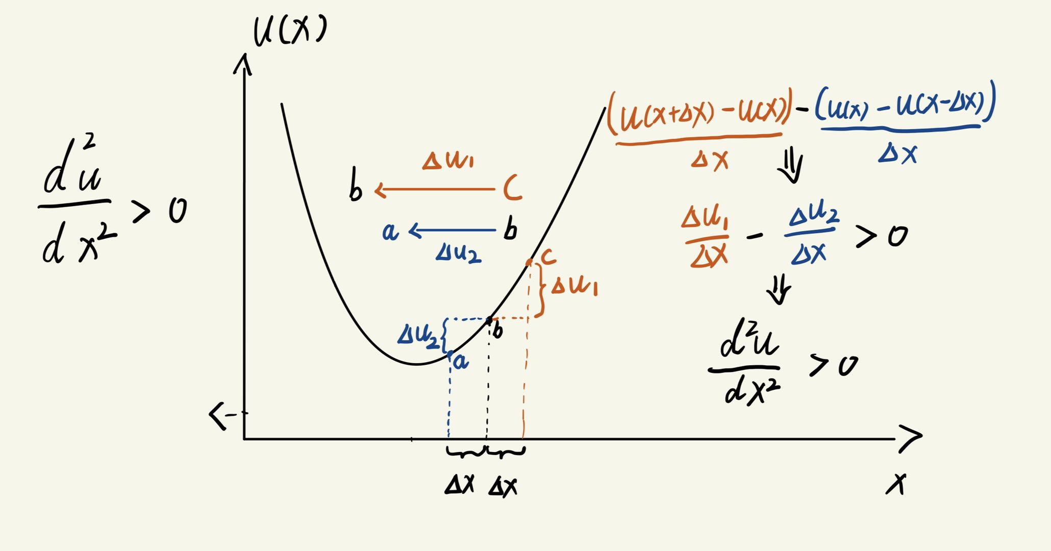 We take the case where the Laplacian is greater than 0 as an example. Suppose $u(x)$ represents the concentration at a specific time $ t$. At the next time step $t+1$ , we expect the concentration to diffuse from regions of higher concentration to lower concentration.
In the figure above, we observe that concentration at point c is higher than at b, and b is higher than a. This means that the substance naturally “flows” from b to a and from c to b. However, since more substance is flowing from c to b than from b to a, the net accumulation at point b increases.
As a result, at the next time step $ t+1$, the concentration at b should be higher than it was at $t$ . In other words, the concentration increases when:
\[\frac{d^2u}{dx^2} > 0\]This demonstrates why a positive Laplacian leads to an increase in concentration at a given point.
3. Discretizing the Diffusion Term
To solve diffusion equations numerically, we discretize the second derivative using the finite difference method. The central difference approximation for$ \frac{d^2u}{dx^2}$ is:
\[\frac{d^2u}{dx^2} \approx \frac{u(x+\Delta x) - 2u(x) + u(x-\Delta x)}{(\Delta x)^2}\]This expression represents the difference of differences, capturing how the concentration changes relative to its neighbors.
In a numerical simulation, we represent space as a grid and update the values using:
\[\frac{\partial u}{\partial t} \approx \frac{u^{n+1}_i - u^n_i}{\Delta t} = D \frac{u^n_{i+1} - 2u^n_i + u^n_{i-1}}{(\Delta x)^2}\]where $ u^n_i $ represents the concentration at grid point $ i$ at time step $ n$ . This allows us to compute diffusion over time.
Pseudocode for Discretization
initialize u[x]  # Define concentration profile on a spatial grid

for each time step:
    for each spatial point i (excluding boundaries):
        # du/dt = D * (u(i+1) - 2u - u(i-1)) / dx^2
        # ( u_new[i] - u[i] )/ dt = D * (u[i+1] - 2*u[i] + u[i-1]) / dx^2
        u_new[i] = u[i] + D * dt / dx^2 * (u[i+1] - 2*u[i] + u[i-1])

    update u with u_new  # Move to the next time step
4. Adding the Reaction Term
To model chemical reactions along with diffusion, we introduce a reaction term $ R(u)$ :
\[\frac{\partial u}{\partial t} = D \frac{\partial^2 u}{\partial x^2} + R(u)\]The reaction term $ R(u)$ represents processes like:
- Chemical transformation (e.g., one substance converting into another),
- Population growth/decay,
- Energy generation or loss in physical systems.
This makes the reaction-diffusion equation a powerful tool in many scientific fields.
5. Full Reaction-Diffusion Equation and Applications
In complex systems, multiple substances interact, leading to coupled equations. The full reaction-diffusion system often takes the form:
\[\frac{\partial u}{\partial t} = D_u \nabla^2 u + f(u, v)\] \[\frac{\partial v}{\partial t} = D_v \nabla^2 v + g(u, v)\]where:
- $u$ and $v$ are interacting chemicals or populations,
- $D_u$ and $D_v$ are their respective diffusion rates,
- $f(u,v)$ and $g(u,v)$ describe their interactions.
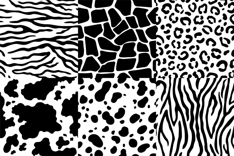
This system explains pattern formation in:
- Animal fur patterns (Turing patterns),
- Coral growth and morphogenesis,
- Flame propagation and reaction fronts.
Key takeaways
- Fick’s Second Law describes diffusion mathematically.
- The second derivative captures how concentration varies relative to neighbors.
- Discretizing the diffusion term allows numerical simulations.
- Adding a reaction term models chemical and biological processes.
☕ Happy learning journey~ 🛠️