Understanding the Diffusion Term (Part II)
In the previous article about the diffusion term, we discussed how to understand the diffusion term from the definition of second derivatives, and introduced how to discretize it for numerical simulation. In this article, we will explore a more general perspective, understanding diffusion from a geometric viewpoint, and explain why people often say that the Laplacian operator is the divergence of the gradient. I will try to explain these concepts in an intuitive way. In this article, I will use a two-dimensional finite volume approach to prove it. This may sacrifice some mathematical rigor, but I think it is very helpful for building intuitive understanding. This line of reasoning can also naturally extend to higher-dimensional cases. I hope this helps everyone better understand these strange “triangle” operators.
Diffusion and Gradient
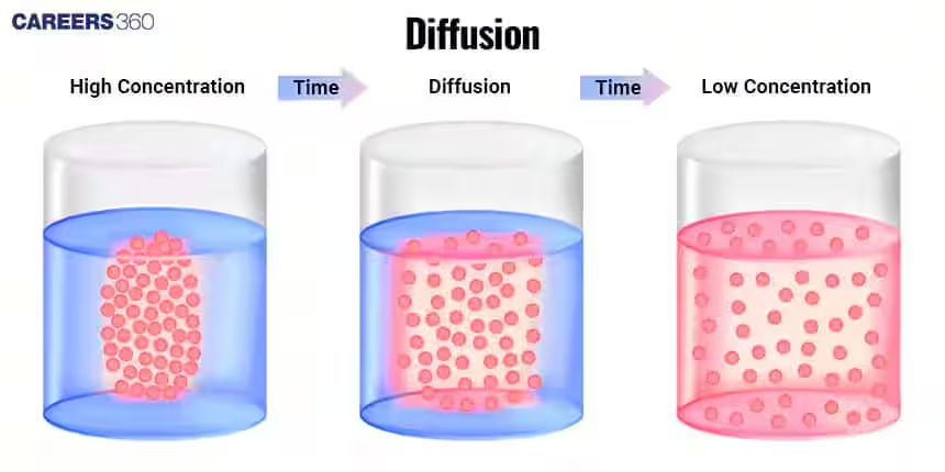 For diffusion phenomena, our intuitive understanding is that substances diffuse from regions of high concentration to regions of low concentration. So at a certain moment and a certain point, we want to describe the direction of material flow. Therefore, we need a mathematical tool to describe this phenomenon. At this point, you may already think of using the gradient, because the gradient vector points in the direction of the fastest increase of the function value (if you are interested in this, you can check my previous article about gradient). Therefore, for a concentration function, we only need to add a negative sign to make the direction point from high concentration to low concentration, and add a diffusion coefficient $D$, and we obtain the flux expression in Fick’s law. In 2D:
Here $\phi$ is some kind of density. As long as a physical quantity exhibits diffusive behavior, we can use this structure to describe its flux. Here flux is a vector, whose direction $\frac{\vec{J}}{|\vec{J}|}$ indicates the direction of material flow, and its magnitude $|\vec{J}|$ represents the amount of material passing through unit area per unit time. For different phenomena, $\phi$ represents different physical quantities:
- For the concentration diffusion we discuss, $\phi$ is concentration, usually denoted as $c$, so the flux is \(\vec{J} = -D \nabla c\)
- In heat conduction phenomena, $\phi$ is temperature, usually denoted as $T$, so the flux is \(\vec{q} = -k \nabla T\) (Fourier’s law)
Therefore, we can see that although these phenomena look very different, their mathematical structures are very similar. This is why we can use the same equation to describe them.
Let us further elaborate on the concept of flux. Flux represents the amount of material passing through unit area per unit time. Its dimension is $[quantity]*[time]^{-1}*[area]^{-1}$. So loosely speaking, once we know the flux at a point, we can multiply the flux by the desired time and area, and obtain the amount of material passing through that area during that time.
Changing Regions and Conservation of Physical Quantities
With the flux $\vec{J}$, we already know the direction and intensity of material flow at a certain point. But information at a certain point is not what we truly care about. What we really care about is:
How does the material concentration inside a small region change over time?
In other words, a region composed of many points is what interests us. According to the conservation principle, the change of material inside a region can only come from inflow or outflow across the boundary. Material will not be created or destroyed out of nowhere inside the region. Therefore, the problem transforms into:
How do we compute the net outward flux across the boundary of the region?
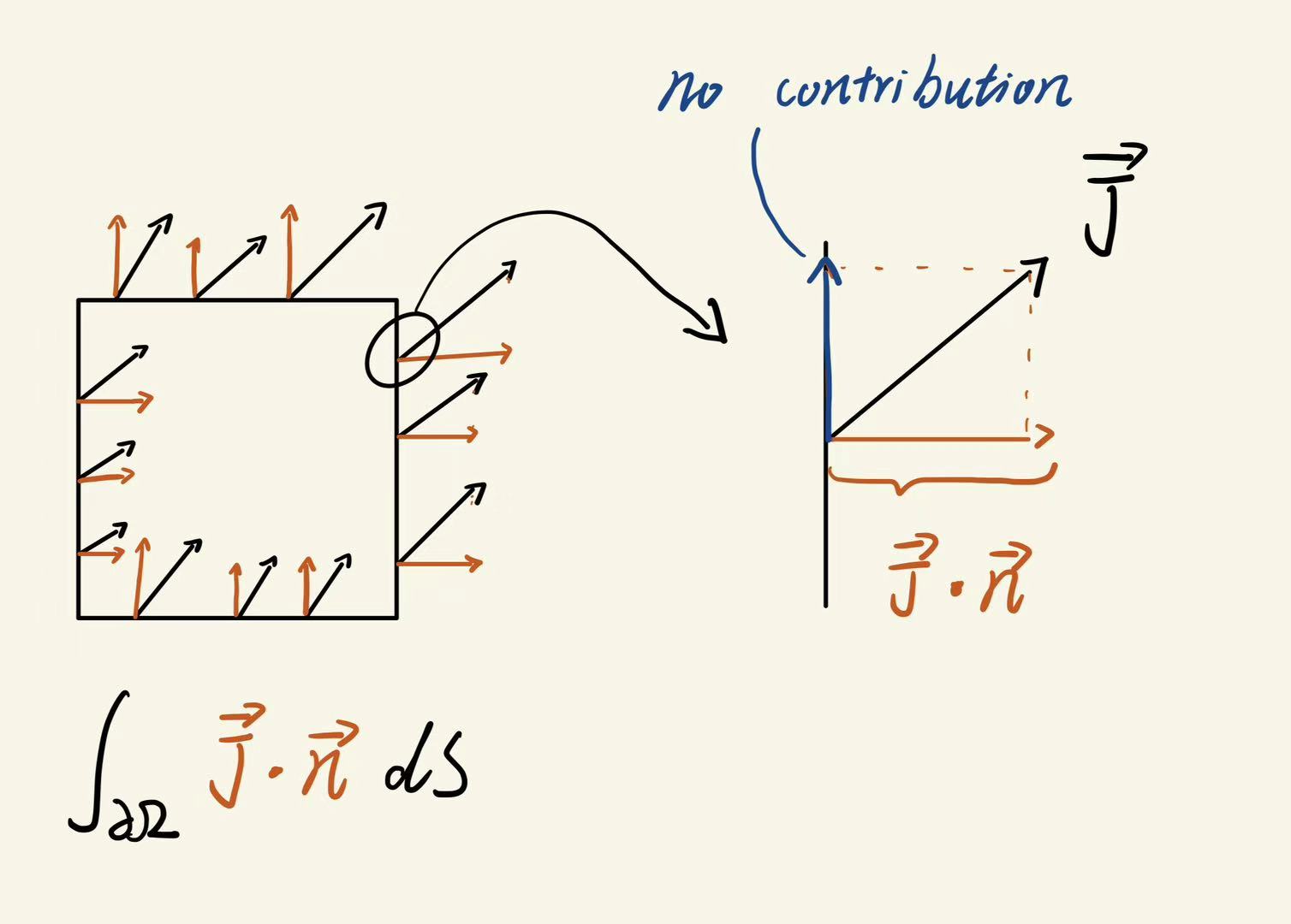
As shown in the figure, we select a small rectangle as the region of interest. The black arrows are the flux vectors at each boundary point, and the boundary is formed by the black edges of the rectangle. A vector can always be decomposed into a normal component and a tangential component. Therefore, we can decompose the flux $\vec{J}$ into the blue tangential component along the boundary and the red normal component perpendicular to the boundary. Only the normal component perpendicular to the boundary will actually pass through the boundary and change the amount of material inside the region. The tangential component along the boundary will not change the material inside the region. Therefore, what we need is the component of $\vec{J}$ in the normal direction:
\[\vec{J} \cdot \vec{n}\]The above expression calculates the contribution of a single point to inflow or outflow of the region. Next, we compute the flux over the entire boundary, so we integrate over the boundary:
\[\int_{\partial \Omega} \vec{J} \cdot \vec{n} \, dS\]Do not be afraid of this integral sign. We can understand it as a summation process. Imagine we divide the boundary into many small pieces. Each small piece has a flux $\vec{J} \cdot \vec{n}$. Adding up the flux on all these pieces gives the net outward flux across the entire boundary. Just like in the figure above, I selected three points on each edge. We can imagine that the more points we take on each edge, the more accurate the calculation becomes. Here $\partial \Omega$ denotes all the boundaries of this small region. For the entire region, we usually denote it as $\Omega$, and $\partial \Omega$ (read as partial $\Omega$, same origin as partial derivative) represents the boundary of this region.
Regarding net outward flux: one important point is why we call it net outward flux. This is because we define the normal vector to point toward the outside of the region. Therefore, if the integral result is positive, it means net outflow; if negative, it means net inflow. If you define the normal vector pointing inward, then the interpretation reverses. This is also why we usually say divergence greater than zero means divergence (spreading out), and divergence less than zero means convergence. Once we change the definition of the normal direction, the interpretation of the result must also change.
Divergence and High-Dimensional Diffusion
The previous step gives the net outward flux for a specific region.
However, what we truly want is not global information dependent on region size, but a description that holds at each point in space.
Therefore, we must normalize this net outward flux to unit area (or volume, depending on dimension), so that it no longer depends on the scale of the selected region, and becomes a local outflow rate. In 2D, the area of the rectangle is $\Delta x \Delta y$, so the outward flux per unit volume is:
\[\frac{1}{\Delta x \Delta y} \int_{\partial \Omega} \vec{J} \cdot \vec{n} \, dS\]When $\Delta x$ and $\Delta y$ approach zero, this expression becomes a limit:
\[\lim_{\Delta x, \Delta y \to 0} \frac{1}{\Delta x \Delta y} \int_{\partial \Omega} \vec{J} \cdot \vec{n} \, dS\]This is exactly the definition of divergence! We replace the flux $\vec{J}$ with a more general vector field $\vec{F}$, and not restrict ourselves to two dimensions. Here $\Delta V$ denotes the volume of the selected region. In 2D, it equals area $\Delta x\Delta y$. We obtain the definition of divergence:
\[\text{div} \vec{F} := \lim_{\Delta V \to 0} \frac{1}{\Delta V} \int_{\partial \Omega} \vec{F} \cdot \vec{n} \, dS\]Next, we will prove how this limit form is equivalent to the familiar divergence expression:
\[\text{div} \vec{F} := \lim_{\Delta V \to 0} \frac{1}{\Delta V} \int_{\partial \Omega} \vec{F} \cdot \vec{n} \, dS= \frac{\partial F_1}{\partial x} + \frac{\partial F_2}{\partial y}\]proof
Readers who do not want to see the proof can skip this subsection.
First, we replace the vector field $\vec{F}$ here with the flux $\vec{J}$ encountered in the diffusion term. Therefore, the integral we need to handle becomes:
\[\int_{\partial \Omega} \vec{F} \cdot \vec{n} \, ds = \int_{\partial \Omega} \vec{J} \cdot \vec{n} \, ds\]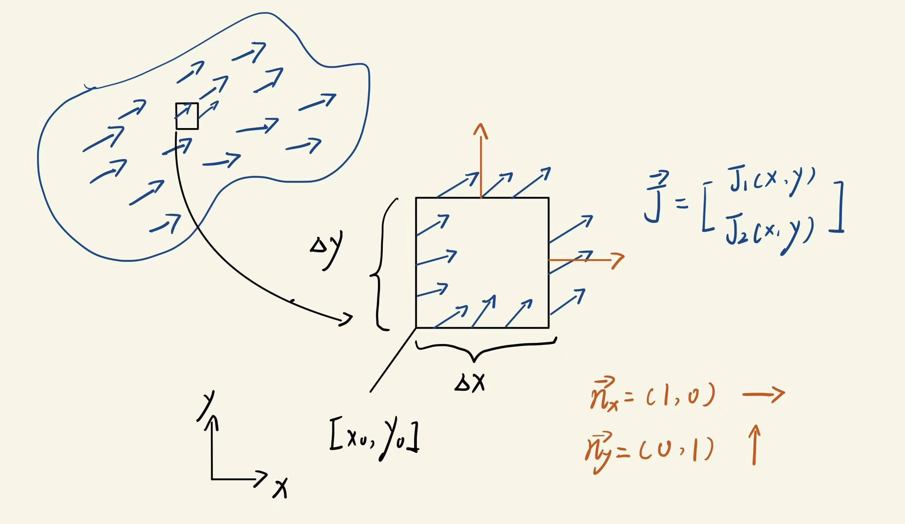
As shown in the figure, we select a small rectangular region from the entire vector field to perform the analysis. We compute the net outward flux on each boundary, and then add them together to obtain the net outward flux across the entire boundary:
\[\int_{\partial \Omega} \vec{J} \cdot \vec{n} \, ds = \int_{x_0}^{x_0+\Delta x} \vec{J}(x, y_0)\cdot (-\vec{n}_y)\, dx + \int_{x_0}^{x_0+\Delta x} \vec{J}(x, y_0+\Delta y)\cdot (\vec{n}_y)\, dx\] \[+ \int_{y_0}^{y_0+\Delta y} \vec{J}(x_0, y)\cdot (-\vec{n}_x)\, dy + \int_{y_0}^{y_0+\Delta y} \vec{J}(x_0+\Delta x, y)\cdot (\vec{n}_x)\, dy\]After taking the dot product with the normal vector on each side, we obtain the parts that contribute to the net outward flux:
\[\int_{\partial \Omega} \vec{J} \cdot \vec{n} \, ds =\int_{x_0}^{x_0+\Delta x}- J_2(x, y_0)\, dx +\int_{x_0}^{x_0+\Delta x}J_2(x, y_0+\Delta y)\, dx\] \[+ \int_{y_0}^{y_0+\Delta y} - J_1(x_0, y)\, dy + \int_{y_0}^{y_0+\Delta y} J_1(x_0+\Delta x, y)\, dy\]Rearranging gives:
\[\int_{\partial \Omega} \vec{J} \cdot \vec{n} \, ds=\int_{x_0}^{x_0+\Delta x} \big[ J_2(x, y_0+\Delta y) - J_2(x, y_0) \big] dx\] \[+\int_{y_0}^{y_0+\Delta y} \big[ J_1(x_0+\Delta x, y) - J_1(x_0, y) \big] dy\]Taking the limit:
\[\lim_{\Delta x, \Delta y \to 0} \int_{\partial \Omega} \vec{J}\cdot \vec{n}\, ds =\lim_{\Delta x, \Delta y \to 0} \left( \int_{x_0}^{x_0+\Delta x} [ J_2(x, y_0+\Delta y) - J_2(x, y_0) ] dx + \int_{y_0}^{y_0+\Delta y} [ J_1(x_0+\Delta x, y) - J_1(x_0, y) ] dy \right)\]Applying the mean value theorem for integrals, and noting that when $\Delta x, \Delta y \to 0$, both $x$ and $y$ approach $x_0$ and $y_0$, we obtain:
\[=\lim_{\Delta x, \Delta y \to 0} \Big( [ J_2(x_0, y_0+\Delta y) - J_2(x_0, y_0) ] \Delta x +[ J_1(x_0+\Delta x, y_0) - J_1(x_0, y_0) ] \Delta y \Big)\]Divide both sides by $\Delta x \Delta y$:
\[\lim_{\Delta x, \Delta y \to 0} \frac{1}{\Delta x \Delta y} \int_{\partial \Omega} \vec{J} \cdot \vec{n} \, ds = \underbrace{ \lim_{\Delta y \to 0} \frac{J_2(x_0, y_0+\Delta y) - J_2(x_0, y_0)}{\Delta y} }_{\text{definition of } \frac{\partial J_2}{\partial y}} + \underbrace{ \lim_{\Delta x \to 0} \frac{J_1(x_0+\Delta x, y_0) - J_1(x_0, y_0)}{\Delta x} }_{\text{definition of } \frac{\partial J_1}{\partial x}}\]Finally, we obtain the definition of divergence:
\[\operatorname{div}\vec{J} := \lim_{\Delta x, \Delta y \to 0} \frac{1}{\Delta x \Delta y} \int_{\partial \Omega} \vec{J} \cdot \vec{n} \, ds = \frac{\partial J_1}{\partial x} + \frac{\partial J_2}{\partial y}\]Finally, we substitute the flux $\vec{J}$ with the expression from Fick’s law $-D \nabla \phi$, and obtain the familiar high-dimensional expression of the diffusion term:
\[\text{div} \vec{J} = \text{div}(-D \nabla \phi) = -D \left( \frac{\partial^2 \phi}{\partial x^2} + \frac{\partial^2 \phi}{\partial y^2} \right) = -D \nabla^2 \phi\]Diffusion Term and Transport Equation
Suppose the physical quantity we want to compute is $\phi$. If we only consider diffusion phenomena, we obtain a pure diffusion equation:
\[\frac{\partial \phi}{\partial t} - D \nabla^2 \phi = 0\]Under this line of reasoning, understanding the transport term becomes very natural. In diffusion phenomena, the driving force of material flow is a vector field related to the gradient, while in transport phenomena, the driving force is a velocity field $\vec{V}$. Therefore, we can understand the transport term as the divergence of a velocity field:
\[\text{div} (\vec{V} \phi)\]Thus, we obtain the equation that simultaneously considers diffusion and transport:
\[\frac{\partial \phi}{\partial t} + \text{div}(\vec{V} \phi) - D \nabla^2 \phi = 0\]When deriving the transport equation, we usually rearrange the diffusion term to the right-hand side. In this way, the negative sign originally present in Fick’s law no longer appears explicitly in the final expression. This also explains a common question: why does the convection term appear in positive divergence form, while the diffusion term ultimately becomes a positive Laplacian operator? Because the flux of convection is $\vec{V} \phi$, so in conservation form it is written as $\text{div}(\vec{V}\phi)$. The flux of diffusion according to Fick’s law is $- D \nabla \phi.$ Therefore, the essential conservation form of the equation is
\[\frac{\partial \phi}{\partial t} + \text{div}(\vec{V}\phi) = - \text{div}(-D\nabla\phi) + S.\]After substituting the diffusion flux and rearranging, the two negative signs cancel, and we obtain the common form:
\[\frac{\partial \phi}{\partial t} + \text{div}(V\phi) = D \nabla^2 \phi + S.\]Here \(S\) denotes the source term. When the transported quantity is replaced by momentum density, and combined with the constitutive relations of fluid stress, we obtain the well-known Navier–Stokes equations (ignoring the continuity constraint).
Key takeaways
- According to Fick’s law, we can use the gradient to describe the flux in diffusion phenomena. Diffusion is driven by the gradient, and matter flows from high concentration to low concentration. Therefore, the flux is $\vec{J} = -D \nabla \phi$.
- According to the conservation principle, the change of material inside a region can only come from inflow or outflow across the boundary. Only the contribution of the normal component changes the material inside the region. Therefore, the net outward flux across the boundary is $ \int_{\partial \Omega} \vec{J} \cdot \vec{n} \, dS $.
- By computing the net outward flux through boundary integration and normalizing it to unit volume, we obtain the definition of divergence. Divergence describes the degree of spreading (net outflow or inflow) of a vector field at each point in space, $\text{div} \vec{F} := \lim_{\Delta V \to 0} \frac{1}{\Delta V} \int_{\partial \Omega} \vec{F} \cdot \vec{n} \, dS$.
- Finally, substituting the flux expression into the divergence definition, we obtain the high-dimensional expression of the diffusion term, proving the connection between the Laplacian operator and diffusion phenomena, $\text{div} \vec{J} = \text{div}(-D \nabla \phi) = -D \nabla^2 \phi$. This is why people often say that the Laplacian is the divergence of the gradient.
☕ Happy learning journey~ 🛠️