Traditional optimization method for continuous optimization
Basic optimization methods
One usually distinguishes between two types of optimization problems: numerical and analytical. However here we disdinguish between unconstrained and constrained optimization problems.
The framework of optimization problems is as follows: given a function $f(x)$, where $x \in \mathbb{R}^n$ or $x$ subject to some constraints like $x$ can only take values in a certain set $X$. The goal is to find the optimal $x$, denoted as $x^*$, that minimizes $f(x)$, namely $f(x^*) = \min_{x \in X} f(x)$.(we only discuss minimization here, but the same applies to maximization by considering $-f(x)$ )
Unconstrained optimization
Gradient descent
Like what I have mentioned in the previous post(click here !), given current point $x_0$, the negitive gradient direction is the direction of the steepest descent. Therefore, we can update the current point by moving in the direction of the negative gradient. The update rule is as follows:
$x_{k+1} = x_k - \alpha\nabla f(x_k)$
where $\alpha$ is the step size, also known as the learning rate. The step size is a hyperparameter that controls the size of the step we take in the direction of the negative gradient. If the step size is too large, we may overshoot the minimum, and if it is too small, the convergence may be slow.
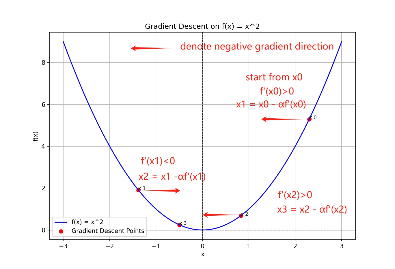
The plot shows a simple example of the gradient descent algorithm. The blue curve represents the objective function, and the red dots represent the steps taken by the algorithm. The algorithm starts at the initial point $x_0$ and moves in the direction of the negative gradient. As it approaches the minimum, it converges to the optimal point $x^* = 0$.
But usually in real life optimization problems, the objective function is not so simple, and the gradient descent algorithm may not be the best choice. For example, the objective function may have multiple local minima, and the gradient descent algorithm may get stuck in a local minimum.
Newton’s method
Newton’s method is another optimization algorithm that uses the not only the first-order information but also the second-order information of the objective function.
$f(x) \approx f(x_0) + \nabla f(x_0)^T (x - x_0) + \frac{1}{2} (x - x_0)^T H(x_0) (x - x_0)$
where $H(x_0)$ is the Hessian matrix, which stored the second-order information of the objective function. It would looks like a little be complicated, but it is actually a generalization of the Taylor expansion.Starting with the one-dimensional case, the equation is reduced to
$ f(x) \approx f(x_0) + f'(x_0)(x - x_0) + \frac{1}{2} f''(x_0)(x - x_0)^2 \equiv f_{[2]}(x) $
Now we use the first and second order information to approximate the objective function, for the approximation function $f_{[2]}(x)$, we can find the minimum by setting the derivative of $f_{[2]}(x)$ to zero.
$f'_{[2]}(x) = 0 \iff f'(x_0) + (x - x_0)f''(x_0) = 0$
Solving this simple equation, one obtains
$x = x_0 - \frac{f'(x_0)}{f''(x_0)}$
And the update rule for the Newton’s method is as follows:
$x_{k+1} = x_k - \frac{f'(x_k)}{f''(x_k)}$
This is the update rule of Newton’s method. Compared to the gradient descent algorithm, Newton’s method converges faster because it uses the second-order information of the objective function. And also the step size $\alpha$ is strictly needed in Newton’s method.
Constrained optimization
Most of the optimization problems occurring in realistic applications are associated with some form of constraints. In such cases, the problem takes the general form
\begin{equation} \begin{aligned} \text{minimize} \quad & f(x) \\ \text{subject to} \quad & g_i(x) \leq 0, \quad i = 1, \ldots, m, \\ & h_i(x) = 0, \quad i = 1, \ldots, k. \end{aligned} \end{equation}
Again, we shall assume that both the objective function and the constraint functions are at least twice continuously differentiable on $\mathbb{R}^n$. In simple cases, a constrained optimization problem can be converted to an unconstrained one
Lagrange multiplier method
Consider a constrained optimization problem with only equality constraints. Simplifying further, let us begin by studying the case $n = 2, k = 1$. In this case, the optimization problem takes the form
\begin{equation} \begin{aligned} \text{minimize} \quad & f(x_1, x_2) \\ \text{subject to} \quad & h(x_1, x_2) = 0. \end{aligned} \end{equation}
We construct a new function $L(x_1, x_2, \lambda)$, where $\lambda$ is a scalar. Define $L(x_1, x_2, \lambda)$ as
\begin{equation} L(x_1, x_2, \lambda) = f(x_1, x_2) + \lambda h(x_1, x_2). \end{equation}
Setting the gradient of $L$ equal to zero, namely all pariial derivatives of $L$ with respect to $x_1, x_2, \lambda$ are zero , we obtain
\begin{equation} \frac{\partial L}{\partial x_1} = \frac{\partial f}{\partial x_1} + \lambda \frac{\partial h}{\partial x_1} = 0, \tag{1} \end{equation} \begin{equation} \frac{\partial L}{\partial x_2} = \frac{\partial f}{\partial x_2} + \lambda \frac{\partial h}{\partial x_2} = 0, \tag{2} \end{equation} \begin{equation} \frac{\partial L}{\partial \lambda} = h(x_1, x_2) = 0. \tag{3} \end{equation}
And then we can solve the above system of equations to find the optimal point $x^*$.
why the Lagrange multiplier method works?
for equation (1) and (2), guarentee that the gradient of the objective function is parallel to the gradient of the constraint function. And why at the optimal point, the gradients are parallel? You can check the link here Geometric Interpretation of the Lagrange Multiplier.
for equation (3), it is the constraint function itself. It is the condition that the optimal point must satisfy.
So the Lagrange multiplier method is a powerful tool that combines the objective function and the constraint function eligantly.
Penalty method
Penalty method can transform a constrained optimization problem to an unconstrained problem that can then be solved using standard numerical methods (such as gradient descent or Newton’s method) for Classical Optimization.
The idea is to add a penalty term to the objective function that penalizes the violation of the constraints, for unequal constraints, we can use the following form:
\begin{equation} \sum_{i=1}^m \max(0, g_i(x))^2 \end{equation}
for equality constraints, we can use the following form:
\begin{equation} \sum_{i=1}^k h_i(x)^2 \end{equation}
So the penalty term would be:
\begin{equation} p(x;\mu) = \sum_{i=1}^m \max(0, g_i(x))^2 + \sum_{i=1}^k h_i(x)^2 \end{equation}
where $\mu$ is a positive parameter (not a variable like the $\lambda$ in the Lagrange multiplier method!). The penalty term is added to the objective function, and the optimization problem becomes
\begin{equation} \text{minimize}\quad f_p(x;\mu) = f(x) + p(x;\mu) \end{equation}
So to minimize the penalty method, the problem is converted to an unconstrained optimization problem. And we can use the gradient descent or Newton’s method to solve it. And as we increase the value of $\mu$, the penalty term will be more and more important, so even a small violation of the constraints will be penalized heavily, and the optimal point will be closer to the feasible region.
Key Takeaways
-
Unconstrained optimization: Gradient descent and Newton’s method are two popular optimization algorithms for unconstrained optimization problems. And gradient descent is a first-order optimization algorithm, while Newton’s method is a second-order optimization algorithm.
-
Constrained optimization: Lagrange multiplier method mainly used to solve optimization problems with equality constraints. And Penalty method can transform a constrained optimization problem to an unconstrained problem that can then be solved using standard numerical methods.
References
- Wahde, M. Biologically Inspired Optimization Methods: An Introduction. Chalmers University of Technology, Sweden, 2008.
☕ Happy learning journey~ 🛠️